What Makes RapidFire AI Different?

The crux of RapidFire AI’s difference is in its adaptive execution engine: it enables “interruptible” execution of configurations across GPUs/CPUs. To do so, it first shards the training and/or evaluation dataset randomly into “chunks” (also called “shards”). Then instead of waiting for a run to see the whole dataset for all epochs (for SFT/RFT) or for full eval metrics calculation (for RAG evals), RapidFire AI schedules all runs on one shard at a time, and then cycles through all shards.

Suppose you have only 1 GPU, say an A100 or H100, and you want to run SFT on a Llama model. Current tools force you to run one config after another sequentially as shown in the (simplified) illustration below. In contrast, by operating on shards, RapidFire AI offers a far more concurrent learning experience by automatically swapping adapters (and base models, if needed) across GPU(s) and DRAM. It does this via efficient shared memory-based caching mechanisms that can spill to disk when needed.

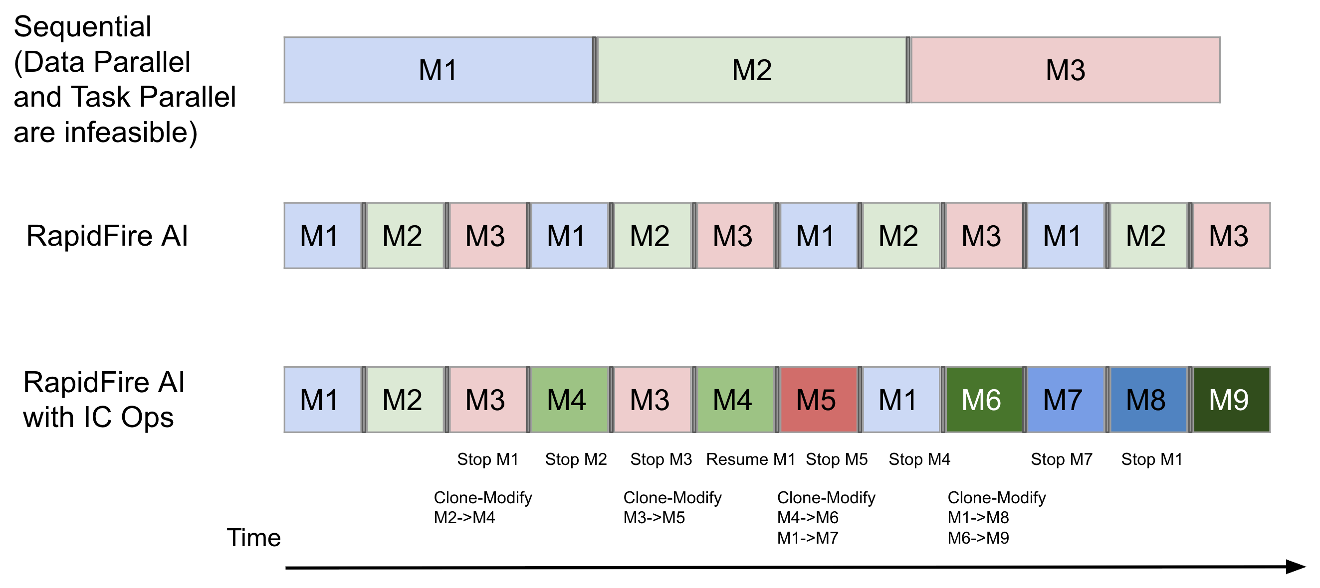
In the above figure, all 3 model configs are shown for 1 epoch. RapidFire AI is set to use 4 chunks. So, before model config 3 (M3) even starts in the sequential approach, RapidFire AI already shows you the learning behaviors of all 3 configs on the first 2-3 chunks. The overhead of swapping, represented by the thin gray box, is minimal, less than 5% of the runtime, as per our measurements–thanks to our new efficient memory management techniques.

For inference evals for RAG/context engineering, such sharded execution means RapidFire AI surfaces eval metrics sooner based on a statistical technique known as online aggregation from the database systems literature. Basically, see estimated values and confidence intervals for all eval metrics in real time as the shards get processed, ultimately converging to the exact metrics on the full dataset.

The Power of Dynamic Real-Time Control

Our adaptive execution engine also enables a powerful new capability: dynamic real-time control over runs in flight. We call this Interactive Control Operations, or IC Ops for short.

Stop non-promising runs at any point–they will be put on a wait queue. Resume any later if you want to revisit it. Clone high-performing runs from the dashboard and Modify the configuration knobs as you see fit to try new variations. Warm start the clone’s parameters with the parent’s to give them a headstart in learning behavior. Under the hood, RapidFire AI automatically manages how runs and chunks are placed on GPUs, freeing you to focus fully on the logic of your AI experiment rather than wrestling with low-level systems issue to parallelize your work.

As the above figure shows, with suitable IC Ops based on the runs’ learning behaviors, you are able to compare 9 configs in roughly the same time it took to compare 3 sequentially! Read more about IC Ops here.

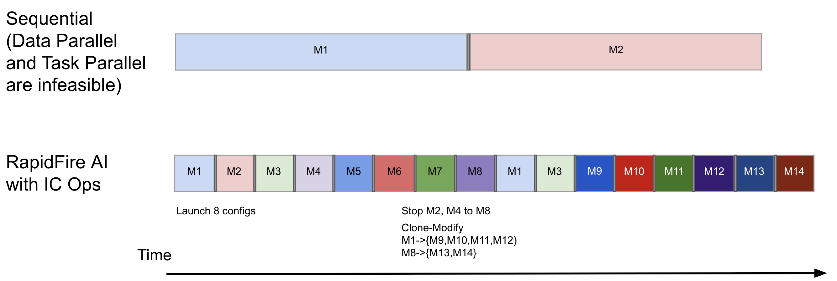
In the second example shown above, we show how you can be even more aggressive with your exploration thanks to RapidFire AI: launching 8 configs together even on just 1 GPU. And with multiple Stop and Clone-Modify operations, you can get a feel for even 14 configs on 1-2 shards each in roughly the time it would take to compare just 2 configs on the full data! All the while, you are free to continue the training of whichever configs still look promising, resume those that you had stopped earlier, clone the clones further, and so on.

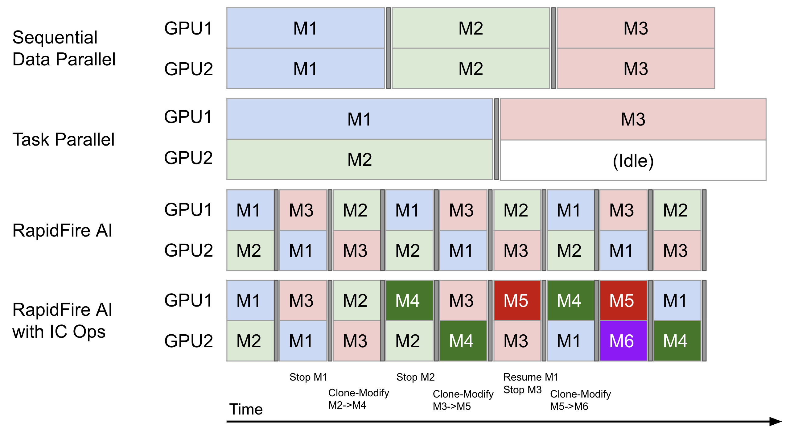
RapidFire AI supports multi-GPU setups natively. Here is a (simplified) illustration of sequential execution with Data Parallelism (say, with DDP or FSDP) vs. Task Parallelism (say, with Weights & Biases) vs. RapidFire AI, both without and with IC Ops. Our scheduler navigates multiple GPUs automatically so that you need not worry if any GPU is underutilized, e.g., like in the case of Task Parallelism for the workload shown below.

Likewise, for RAG/context engineering evals on self-hosted LLMs, the above multi-GPU scheduling optimizations also apply out of the box, albeit analogous to a single epoch. When using only closed model APIs such as OpenAI, RapidFire AI’s scheduler automatically optimizes how CPU cores and the token rate limits are apportioned across configs. This will help avoid wastage of token spend on unproductive RAG configs and help you redirect the spend to more productive RAG configs in real time.

Why Not Just Downsample Data?

At first glance, one might consider running multi-config comparisons by downsampling data for quick estimates, then running promising configs on full data. While common, this approach is often misleading and cumbersome.

A single downsample introduces variance from one static snapshot, potentially leading to wrong conclusions, especially with overfitting-prone LLMs/DL models. It requires manual checkpoint management, adding tedious file work. You also do not get dynamic control (stop, resume, clone-modify), or you must reimplement such tricky operations, taking time away from your AI application work.

RapidFire AI takes such practical heuristics to their logical conclusion with shard-based adaptive multi-config execution with dynamic experiment control. This offers you maximum power and flexibility for AI development without extra DevOps grunt work, i.e., rapid experimentation.

The above said, note that downsampling is complementary to rapid experimentation–feel free do both! The adaptive execution can operate on your downsampled dataset all the same.